

Demography is Not Destiny
Part 1: Age Structure and Crime

The following is an excerpt of a chapter intended to be part of a book that I am in the process of writing. Constructive feedback on this excerpt is welcome.
Hypothesized Association: Age Composition and Homicide Trends
Given the consistency of this age-graded pattern in offending in the United States, some have claimed that the age composition of the population could impact the crime rate. That is, all else being equal, the greater the percentage of the population composed of people in their peak offending ages (~15-24), the higher the rate of crime. Because crime statistics are standardized by population size, a high percentage of the population being comprised of teenagers and young adults would be expected to make the baseline crime rate (per capita) higher.
The age composition impact became relevant to conversations about post-World War II crime trends due to the abnormally large ‘Baby Boomer’ cohort. Prior to World War II, fertility rates had been declining. During and after the war, the fertility trend abruptly reversed itself, as women roughly doubled their fertility rate from 1939 (77.6 per 1,000 women 15-44) to 1957 (122.9 per 1,000).[1] This baby ‘boom’ was believed to be a harbinger of criminological doom in the coming decades as these children aged into their teens and early 20s. If the typical age and crime patterns held, this growing cohort could result in an alarming increase in crime.
A related argument by Richard Easterlin[2] suggests that larger youth cohorts are related to various social problems. Easterlin makes a neo-Malthusian argument about population size and relative scarcity of resources. In effect, in larger cohorts, young people are in “over-supply” contributing to higher youth unemployment, higher rates of consumer inflation, more political alienation and, notably, an increase in the homicide rate. Citing a potential decline in relative income, Easterlin suggests that crime, and specifically homicide, increased as a result of the Baby Boomer cohort. Easterlin’s argument suggests that not only will the crime rate be impacted by more youth due to population composition, but also that the youth of large cohorts will be more prone to commit crime than the youth of smaller cohorts.
The overall claim examined in this chapter is that population demographics impact homicide rate trends. That is, a more youthful population will result in a higher homicide rate. The more specific claim about post-World War II crime trends is that the increase in homicide was due to Baby Boomers - that there were so many young people in the late 1960s and 1970s that crime rates increased as a result.
Evidence for the Age-Composition Argument
An initial glance at the overarching evidence would suggest that larger youth populations contribute to higher rates of homicide. There was a sharp increase in all types of crimes during the 1960s and 1970s,[3] which happened to correspond with when the Baby Boomer cohort was hitting peak crime ages. During the second half of the 20th Century, the highest rate of homicide was recorded in 1980.[4] This peak in the homicide rate occurred 23 years after the largest post-War cohort was born (1957), which suggests that there were simply more teens and young adults in the population, resulting in a high rate of crime.
Probably the most convincing argument for the Baby Boomer-induced crime wave was the correspondence of these trends as highlighted by Lawrence Cohen and Kenneth Land.[5] Using demographic data (percentage aged 15 to 29) along with a few other control variables, Cohen and Land were able to trace the rise and fall of crime trends from 1946 to 1984. Although their model did not anticipate the mid-1980s reversal of the decline (increase) in the homicide trend, their overall predictions that crime rates would fall into the 1990s and early 2000s would be largely vindicated by the data in the coming decades.
Easterlin’s[6] observations and predictions also corresponded with these general trends. Examining roughly the same time span, Easterlin showed that the rise in homicide corresponded with the larger Baby Boomer cohort.
The figure below (Figure 3.2) depicts the percentage of the population aged 15 to 24 alongside the homicide rate from 1946 to 2024. In general, these trends move together fairly closely (r = .64). Much like it was documented by Easterlin as well as Cohen and Land, there is a sharp increase in homicide during the 1960s and 1970s that roughly corresponds with the increase in the youth and young adult population.
Figure 3.2.
Percentage Aged 15 to 24 and the Homicide Rate per 100,000, 1946-2024.
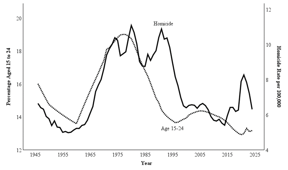
However, the correspondence of these trends after 1980 is a bit more ‘mixed.’ There was an abrupt increase in homicide from 1985 to 1991 that occurred at the same time that the proportional share of the youth and young adult population (15-24) was shrinking. Additionally, the homicide spike from 2015 to 2021 was not accompanied by a significant increase in the percentage of the population aged 15 to 24.
Evidence against the Age-Composition Argument
One of the main points of evidence against the age-structure and crime hypothesis stems from the apparent disjuncture of these post-1985 trends. Most infamously, James Fox[7] used similar demographic data concerning the size of the youth population to incorrectly forecast a homicide increase at the precipice of the largest sustained decrease in homicide of the 20th Century. All else being equal, Fox projected that the high rates of violence during the late 1980s and early 1990s would continue, even increasingly slightly alongside increases in the youth population. This time, the predictions using demographic data were very wrong; the 1990s crime decline represented the largest sustained downward trend in homicide of the past 75 years at the same time that the youth population was growing.
One errant prediction does not necessarily mean that we need to “throw the baby out with the bath water,” or, in this case, throwing the criminal contributions of a large cohort of babies out of the crime forecasting equation. The problem with Fox’s forecast was not (necessarily) that age composition of the population has no impact on the crime rate, but that other elements of youth criminality need to be considered. Namely – the impact of ‘period’ and ‘cohort’ effects.
‘Period’ effects refer to characteristics of a given time period/era that contribute to variation in crime; some periods may generally be more criminogenic than others for people of all ages. ‘Cohort’ effects refer to variation in crime attributed to a specific cohort that is more (or less) prone to criminal behavior than other cohorts. As it turns out, the youth of the late 1980s and early 1990s were especially prone to violence during their teen years. Subsequent research suggests that this was likely due to a ‘period’ effect[8] as the arrest rates for violent offenses among the youth of the late 1980s and early 1990s were similar to other cohorts as they aged.[9]
By disaggregating the homicide trend by arrests, we start to see why the demographic predictions failed after the mid-1980s. Prior to that time, every indication was that more youth = more crime. From roughly 1985 onward, youth have played a much larger role in homicide arrests and victimization than during previous eras - even as their relative composition has declined.
In general, we would expect the percentage of arrests attributed to people aged 15 to 24 to track this age group’s composition in the general population. However, as is apparent in Figure 3.3, this has not been the case. The percentage of murder arrests attributed to young (15-24) offenders has been higher than expected since the mid-1980s.
Figure 3.3
Percentage Aged 15 to 24 and their Percentage of Murder Arrests, 1946-2024.
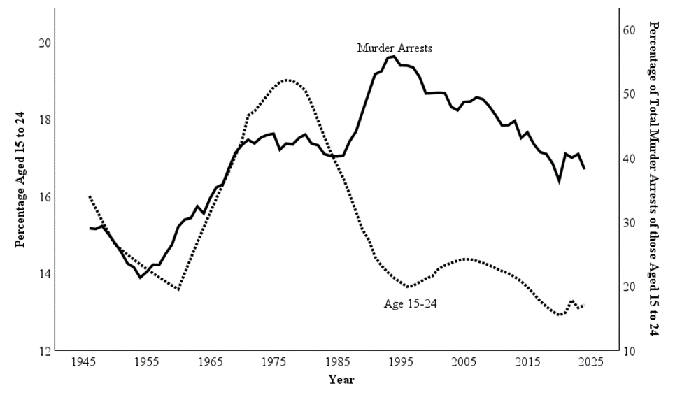
After the ‘Baby Boom’ era, there is little indication that the size of the youth cohort is associated with youth offending or victimization. In fact, there is almost no correlation between the youth/young adult (15-24) composition of the population and their relative composition of the total murder arrests (r = .01) or composition of homicide victims (r = -.02) from 1946 to 2024.[10]
Further, the over-representation of youth does not appear to increase their involvement in crime above baseline levels. Previously, Robert O’Brien[11] drew the conclusion that there was little consistent support for Easterlin’s hypothesis on murder trends specifically. O’Brien found that cohort size seemed to be more consistently related to property-based offenses rather than aggravated assault and murder.[12]
With more contemporary data, it is apparent that Easterlin’s hypothesis - that large youth cohorts are more prone to crime - is the opposite of what has occurred since the mid-1980s. As youth cohort shrank, their over-representation in homicide arrest and victimization statistics has increased. In fact, the Baby Boomer cohort did not appear to be over-represented in homicide involvement, and is even less over-represented than all subsequent cohorts.
In Figure 3.4, I present these trends. The metric used in this figure is the percentage of murder arrests and homicide victimization for those aged 15 to 24 divided by the percentage of the population aged 15 to 24. The period between 1965 and 1985 is shaded to represent the era in which Baby Boomers, the largest post-World War II birth cohort, were in their prime offending years. There appears to be a marginal increase in youth over-representation in homicide arrest and victimization statistics as Boomers reached peak crime-involvement ages, which is likely why the Easterlin hypothesis appeared to be plausible. However, since the Baby Boomer cohort, the over-representation of youth among homicide involvement statistics has consistently been higher. The over-representation of youth in murder arrests increased by nearly 68% from 1985 to 1994, just as the proportion of youth in the population were plummeting.
Figure 3.4
Percentage Aged 15 to 24 Over-Representation of Murder Arrests and Homicide Victimization, 1946-2024.
Evaluation of Age Composition on Homicide Trends
Logically, it would make intuitive sense that a more youthful population structure to contribute to higher rates of crime. After all, despite considerable changes in homicide offending and victimization since World War II, the peak age of arrest has consistently remained between 18 and 24. All else being equal, we would expect there to be a higher murder rate when the population was comprised of a greater proportion of people in this age range.
Yet, all else is not equal over time. The expansion of the use of age-period-cohort models is an implicit acknowledgement that age is just one factor shaping criminal involvement that might not be able to tell us much on its own. Accordingly, a simple examination of the relative youthfulness of the population will tell us little about the homicide trend over time. The strongest evidence for the age-composition argument, the relatively strong bivariate correlation with the overall homicide rate (r = .62). However, this appears to be an illusion as the youth composition of homicide victims and offenders does not follow the youth population composition trend.
Population composition likely plays some role, but not as large as previously believed. For example, having a more youthful age-structure likely increases the ‘upper limit’ of the aggregate high homicide rate. And, if the more-homicide-prone recent cohorts[13] since the mid-1980s were larger, the homicide rate would also be higher as well. Yet, simply following trends in the percentage of the population in peak crime ages will likely tell you little about the direction of the homicide trend, especially in the short term. Similar to Robert Sampson’s[14] arguments concerning individual-level risk factors and social change, people who are young are more prone to offending and victimization than those older, but the impact of youth changes alongside social context.
Conclusion
The age composition of the population can probably set our expectations, but is not all that reliable in helping us predict where the homicide trend is going. Given the trends prior to the mid-1980s, the age-composition impact was probably helpful in this regard. However, in more recent cohorts, youth and young adults are apparently more prone to involvement in violence. Accordingly, we would need to periodically recalibrate our expectations about youth contribution to homicide offending to accurately predict homicide trends by simply looking at age composition.
Taken together, I would rate the impact of youth composition of the population as relatively poor in helping us understand post-World War II homicide trends in the United States, especially after the mid-1980s. To contravene an often-referenced quote attributed to the sociologist Auguste Comte, demography is not destiny when it comes to American homicide trends.
[1] National Center for Health Statistics. (2018). Natality trends in the United States, 1909-2018. https://www.cdc.gov/nchs/data-visualization/natality-trends/index.htm
[2] Easterlin, R. (1978). What will 1984 be like? Socioeconomic implications of recent twists in age structure. Demography, 15(4), 397-432.
[3] Cohen, L., & Felson, M. (1979). Social change and crime rate trends: A routine activity approach. American Sociological Review, 44(4), 588-608.
[4] Centers for Disease Control (2026). National center for health statistics: Mortality data on CDC Wonder. https://wonder.cdc.gov/deaths-by-underlying-cause.html
[5] Cohen, L., & Land, K. (1987). Age structure and crime: Symmetry versus asymmetry and the projection of crime rates through the 1990s. American Sociological Review, 52(2), 170-183.
[6] See footnote 9.
[7] Fox, J. (1997). Trends in juvenile violence. Bureau of Justice Statistics. https://bjs.ojp.gov/library/publications/trends-juvenile-violence
[8] O’Brien, R. (2019). Homicide arrest rate trends in the United States: The contributions of periods and cohorts (1965-2015). Journal of Quantitative Criminology, 35, 211-236.
[9] Lu, Y., & Luo, L. (2021). Cohort variation in U.S. violent crime patterns from 1960 to 2014: An age-period-cohort-interaction approach. Journal of Quantitative Criminology, 37, 1047-1081.
[10] It should be noted that prior to 1960, the murder counts and arrests included murders due to ‘negligence’ as well as ‘murder and non-negligent manslaughter.’ Additionally, between 1951 and 1959, the age and arrest data only covered arrests made in large metropolitan cities. However, these changes in data collection do not appear to impact the over-arching conclusion that arrests for murder among young people (15-24) has remained elevated above what would be expected given their relative population size.
[11] O’Brien, R. (1989). Relative cohort size and age-specific crime rates: An age-period-relative-cohort-size model. Criminology, 27(1), 57-78.
[12] See also: Steffensmeier, D., Streifel, C., & Shihadeh, E. (1992). Cohort size and arrest rates over the life course: The Easterlin hypothesis reconsidered. American Sociological Review, 57(3), 306-314.
[13] See also: O’Brien, R. (2019). Homicide arrest rate trends in the United States: The contributions of periods and cohorts (1965-2015). Journal of Quantitative Criminology, 35, 211-236.
[14] Sampson, R. (2026). Marked by time: How social change has transformed crime and the life trajectories of young Americans. Harvard University Press.